Execution Plans

What is deferred compilation?

When I talked about row estimations for table variables, I mentioned ‘deferred compile’, but didn’t give a whole lot of details. What, then, is a deferred compilation? Let’s start with how batches work normally.

T-SQL is an interpreted language. While we talk about compiles, they’re not compilations in the sense of what happens to C++. There’s no conversion of the script to a machine language or intermediate language which is used from that point onwards. Every time a batch executes, it has to be parsed, bound and have an execution plan generated or fetched from cache.

When a batch is parsed, the entire batch is parsed.

SET STATISTICS TIME ON
GO

SELECT * FROM dbo.Clients

SELECT * FROM dbo.StarSystems ss 
INNER JOIN dbo.Stations s ON s.StarSystemID = ss.StarSystemID

SELECT GETDATE()
GO

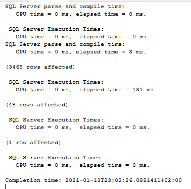
Ignoring the SET STATISTICS, we’ve got there one batch with two queries in it. Two queries, two execution times but only one parse and compile time. The entire batch was compiled and then the batch was executed.

If we set up an XE session to track compiles, it shows similar

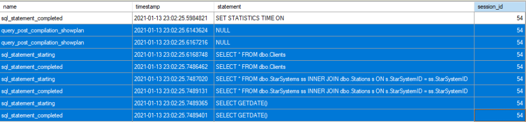
The XE session shows that the compilations for both queries were completed before either started execution.

But what happens if we reference a table that doesn’t exist?

SET STATISTICS TIME ON
GO

SELECT * FROM dbo.Clients

SELECT * FROM dbo.StarSystems_DoesNotExist ss 
INNER JOIN dbo.Stations s ON s.StarSystemID = ss.StarSystemID

SELECT GETDATE()
GO

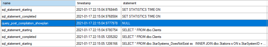
The first of the queries is still compiled, but not the second. The second can’t be compiled because it references an object that doesn’t exist. The first query then executes, and right before when the second query would execute, it’s sent back to be bound and optimised. In this case, the object still doesn’t exist and so we get an error.

Msg 208, Level 16, State 1, Line 6
Invalid object name 'dbo.StarSystems_DoesNotExist'
.

But if the object was created between the start of the batch and the query that uses it, we get a still different result

SET STATISTICS TIME ON
GO

SELECT * FROM dbo.Clients

SELECT * INTO #StarSystems FROM dbo.StarSystems

SELECT * FROM #StarSystems ss 
INNER JOIN dbo.Stations s ON s.StarSystemID = ss.StarSystemID

SELECT GETDATE()
GO

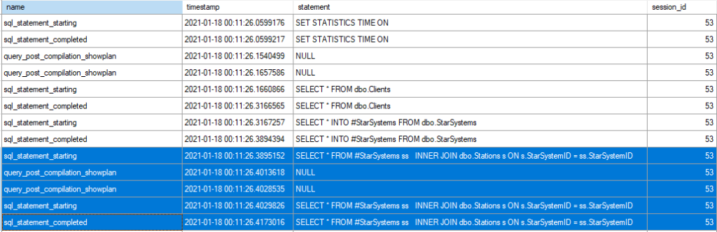
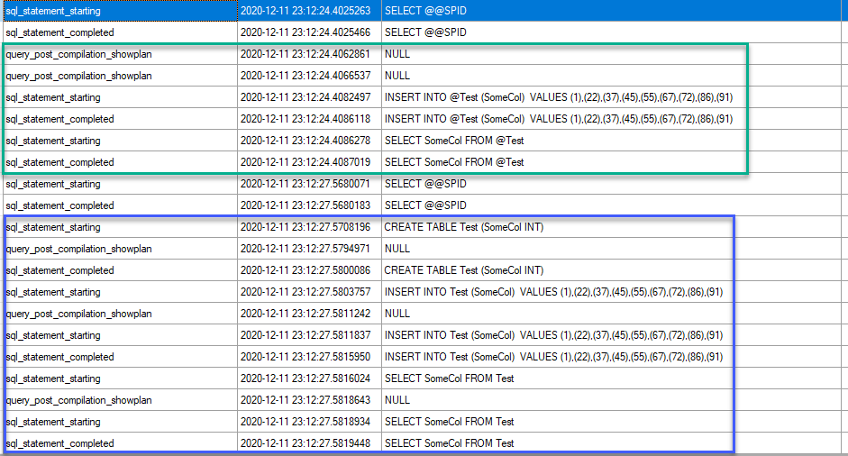
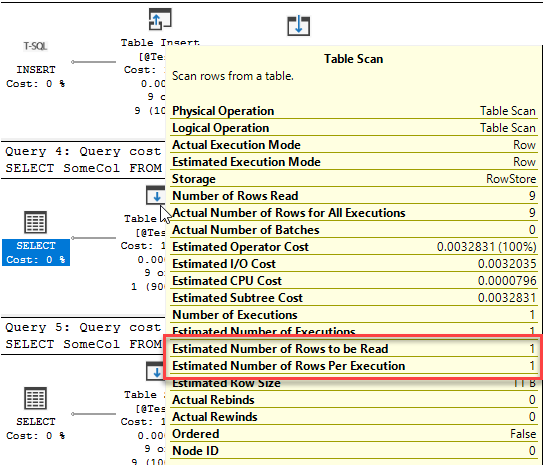
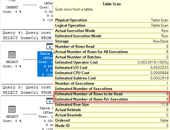
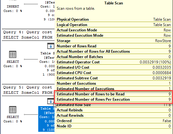
This time we have three queries. Two of them get an execution plan generated when the batch starts, but the third can’t, because the table it references doesn’t exist. Instead, the statement starts executing but can’t execute because there’s no plan. It gets sent back to the optimiser to be compiled, then the query executes.

This is a deferred compile (also called deferred resolution). A compile that does not happen when the batch starts, but is rather deferred until the point that the query itself executes, usually because the table does not exist at the point the batch starts..

On table variable row estimations

At first glance, the question of how many rows are estimated from a table variable is easy.

But, is it really that simple? Well, not really. To dig into the why, first we need to identify why table variables estimate 1 row. The obvious answer is because they don’t have statistics. However…

ALTER DATABASE CURRENT SET AUTO_CREATE_STATISTICS OFF
GO

CREATE TABLE Test (SomeCol INT);

INSERT INTO Test (SomeCol)
VALUES (1),(22),(37),(45),(55),(67),(72),(86),(91)

SELECT SomeCol FROM Test

SELECT * FROM sys.stats WHERE object_id = OBJECT_ID('Test')

DROP TABLE dbo.Test

That table has no statistics, but it still estimates rows correctly.

So it’s not just the absence of statistics. Hmmm… Where else is there a difference with a table variable?

It has to do with when the plans are generated. The XE event results are from an event tracking statement start and end and the post-compilation event for the plan. For the query using the table variable, the entire batch is compiled before the execution starts. For the permanent table, there are multiple compilation events.

And this is because of something called ‘deferred compile’. For the table variable, the entire batch is compiled at the start, at a time where the table variable does not exist, and because there are no statistics, no recompile is triggered after the insert. Hence, there cannot be any row estimation other than 1 row, because the table did not exist when the estimate was made.

For the permanent table, the compilation of the query that uses the table is deferred until the query starts, not when the batch starts. Hence the plan for the query is generated after the table exists, after it’s been populated. That’s the difference here.

Now, there’s still no statistics, and so there’s no way to get data distribution, but that’s not the only way to get information on the rows in the table. The Storage Engine knows how many rows are in the table, though data distribution isn’t known.

Hence, with a table variable we can expect to see an estimated row count other than 1 any time the table variable exists before the query that uses it is compiled.

That will happen when the table variable is a table-type parameter, when the query using it has the RECOMPILE option, and when SQL 2019’s deferred compile for table variables is in play.

CREATE OR ALTER PROCEDURE TestRowEstimations @Input TestTableType READONLY AS

SELECT SomeCol FROM @Input;

DECLARE @Test TABLE (SomeCol INT);

INSERT INTO @Test (SomeCol)
VALUES (1),(22),(37),(45),(55),(67),(72),(86),(91);

SELECT SomeCol FROM @Test;

SELECT SomeCol FROM @Test OPTION (RECOMPILE);
GO
Table-valued parameter
Normal select on compatibility mode 140
Normal select on compatibility mode 150
Select with OPTION(RECOMPILE)

A new way of getting the actual execution plan

Getting the actual execution plan, that is the plan with run-time statistics for a query from an application has always been a little difficult. It’s fine if you can get the query running in Management Studio and reproducing the behaviour from the app, but that can be difficult.

There’s the query_post_execution_showplan event in Extended Events, but that’s a pretty heavy event and not something that I’d like to run on a busy server.

No more! SQL 2019 adds a new plan-related function to get the last actual plan for a query: sys.dm_exec_query_plan_stats.

The function is not available by default, Last_Query_Plan_Stats database scoped configuration has to be set  to allow it to run, and it’s going to add some overhead, how much is still to be determined.

ALTER DATABASE SCOPED CONFIGURATION SET LAST_QUERY_PLAN_STATS = ON

It’s a function which takes a parameter of a plan handle or a sql handle. Hence it can be used alone, or it can be on the right-hand side of an apply from any table or DMV that has a plan handle or sql handle in it. As an example it can be used with QueryStore.

WITH hist
AS (SELECT q.query_id, 
           q.query_hash,
           MAX(rs.max_duration)  AS MaxDuration
    FROM 
        sys.query_store_query q INNER JOIN sys.query_store_plan p ON q.query_id = p.query_id
        INNER JOIN sys.query_store_runtime_stats rs ON p.plan_id = rs.plan_id
        INNER JOIN sys.query_store_runtime_stats_interval rsi ON rs.runtime_stats_interval_id = rsi.runtime_stats_interval_id
    WHERE start_time < DATEADD(HOUR, -1, GETDATE())
    GROUP BY q.query_id, query_hash),
recent
AS (SELECT q.query_id, 
           q.query_hash,
           MAX(rs.max_duration)  AS MaxDuration
    FROM 
        sys.query_store_query q INNER JOIN sys.query_store_plan p ON q.query_id = p.query_id
        INNER JOIN sys.query_store_runtime_stats rs ON p.plan_id = rs.plan_id
        INNER JOIN sys.query_store_runtime_stats_interval rsi ON rs.runtime_stats_interval_id = rsi.runtime_stats_interval_id
    WHERE start_time > DATEADD(HOUR, -1, GETDATE())
    GROUP BY q.query_id, query_hash),
regressed_queries 
AS (
    SELECT hist.query_id, 
            hist.query_hash
        FROM hist INNER JOIN recent ON hist.query_id = recent.query_id
        WHERE recent.MaxDuration > 1.2*hist.MaxDuration
    )
SELECT st.text, OBJECT_NAME(st.objectid) AS ObjectName, qs.last_execution_time, qps.query_plan
    FROM sys.dm_exec_query_stats qs 
        CROSS APPLY sys.dm_exec_sql_text (qs.sql_handle) st
        OUTER APPLY sys.dm_exec_query_plan_stats(qs.plan_handle) qps
    WHERE query_hash IN (SELECT query_hash FROM regressed_queries)

The above query checks query store for any query that has regressed in duration in the last hour (defined as max duration > 120% of previous max duration) and pulls the last actual plan for that query out.

And a look at that plan tells me that I have a bad parameter sniffing problem, a problem that might have been missed or mis-diagnosed with only the estimated plan available.

Comparing plans in Management Studio

Previously I looked at using Query Store to compare execution plans, but it’s not the only way that two execution plans can be compared. The other method requires a saved execution plan and the Management Studio execution plan viewer.

Let’s start by assuming I have a saved execution plan for a query and I want to compare it to the execution plan that the same query currently has. First step is to run the query with actual execution plan on. Right-click on the execution plan and select ‘Compare Showplan’

ComparePlans2

Pick a saved execution plan. It doesn’t have to be for the same query, but the comparison will be of little use if the two plans being compared are not from the same query.

ComparePlansFindPlan

And then we get the same comparison screen as we saw last time with the comparison via Query Store. Similar portions of the plan are marked by coloured blocks, and the properties window shows which properties differ between the two plans.

ComparePlansDetail2

Comparing plans in Query Store

One feature that was added in the 2016 version of SSMS that hasn’t received a lot of attention, is the ability to compare execution plans.

There’s two ways of doing this, from Query Store and from saved files.

Let’s start with Query Store, and I’m going to use a demo database that I’ve been working on for a few months – Interstellar Transport (IST). I’ve got a stored procedure in there that has a terrible parameter sniffing problem (intentionally). I’m going to run it a few times with one parameter value, then run it a few more times with another parameter value, remove the plan from cache and repeat the executions in the reverse order.

With that done, the query should show up in the ‘Queries with High Variance’ report (SQL 2017)

image

image

The query has the two expected plans, and they are quite different from each other.

Plan1

Plan2

I can click on the points on the graph individually to see the plans, but comparing the plans in that way is difficult and requires that I make notes somewhere else. What I can do instead is select two different points on the graph and chose the ‘compare plans’ option.

image

This brings up a window where the two plans are displayed one above the other, and areas in the plan which are similar are highlighted.

image

Select an operator and pull up the properties, and the properties of the operator from both plans are shown, with the differences highlighted.

image

This isn’t the only way to compare query plans. The next post will show how it can be done without using Query Store at all.

When a forced plan isn’t forced

One of the uses for the Query Store, added in SQL 2016, is to force plans. Once forced, plans are supposed to remain unchanged, however there are cases where a forced plan will not be applied and a new plan will be generated.

Statistics changes, which are one of the things that usually cause recompiles, don’t disable a forced plan. It would be kinda weird if it did and against the point of a forced plan.

Schema changes are another matter.

Let’s look at a couple of cases.

First, schema changes that make the plan invalid, in other words, schema changes that affect something that the plan explicitly references. There aren’t that many schema changes that can make the plan invalid without making the query invalid as well, but there are a couple. Index changes, for example.

I want to test a few things:

  • An index change that won’t make the plan invalid (eg adding a column)
  • An index change that does make the plan invalid (eg removing a column that the query needs)
  • Renaming the index without changing its definition
  • Adding an index that would be better for the query than the one referenced by the forced plan.

First, the setup. My Interstellar Trading database with an extra index added:

CREATE INDEX idx_ForcingTest on Shipments (ClientID, HasHazardous, HasLiveStock, HasTemperatureControlled)

The query I’ll be running to test is

DECLARE @Storage TABLE (ID INT, Priority TINYINT, CountShipments INT);

INSERT INTO @Storage
SELECT OriginStationID, Priority, COUNT(*) FROM Shipments WHERE ClientID = 17 AND HasHazardous = 1
GROUP BY OriginStationID, Priority
GO

It’s inserting into a table variable to prevent any problems with the resultsets in SSMS.

I’ve been running the query for a while, and its plan is forced.

image

First test:

CREATE INDEX idx_ForcingTest ON Shipments (ClientID, HasHazardous, HasLiveStock, HasTemperatureControlled, ReferenceNumber)
WITH (DROP_EXISTING = ON)

image

No change. Forced plan is still forced.

Now, let’s make that index less useful, by removing a column that the query does need. There’s a key lookup in the plan, so there is a way for the column to be obtained, but it would change what columns come from each operator and where the filters are being done. Same plan shape, but different details.

CREATE INDEX idx_ForcingTest ON Shipments (ClientID)
WITH (DROP_EXISTING = ON)

image

We get a new plan. The forced one is invalid, because the index no longer allows for the seek predicates defined in the plan, and so the forcing is ignored and we get a new plan.

The query still runs without error, which is better than we’d have had using the old USE PLAN hint.

Once I revert the index back to its original definition, the forced plan starts being used again.

How about renaming the index? Since the plan references the index by name, this will probably also cause the plan forcing to fail.

And indeed it does.

image

One last test. I’m going to rename the index back to its old name, and then add a new one that’s better for the query than the index referenced in the forced plan.

image

And we’re still using the forced plan. The addition of a new index did not invalidate the existing plan, and hence the forced plan will still be used, even when there’s a better index.

This is the reason why I recommend using plan forcing only to fix stuff that’s broken in prod, and to find a solution without forced plans for the long term. It’s not always possible but where it is I’d prefer not to leave the plan forcing in place, because it does mean that new indexes are not considered. Plus, if the query store is ever cleared, the forced plan (along with the forcing) are gone.

Obsessing over query operator costs

A common problem when looking at execution plans is attributing too much meaning and value of the costs of operators.

The percentages shown for operators in query plans are based on costs generated by the query optimiser. They are not times, they are not CPU usage, they are not IO.

The bigger problem is that they can be completely incorrect.

Before digging into the why of incorrect percentages, let’s take a step back and look at why those costs exist.

The SQL query optimiser is a cost-based optimiser. It generates good plans by estimating costs for each query operator and then trying to minimise the total cost of the plan. These costs are based on estimated row counts and heuristics.

The costs we see in the query plan are these compilation time cost estimates. They’re compilation-time estimations, which means that they won’t change between one execution of a query using a particular plan and another query using the same plan, even if the parameter values are different, even if the row counts through the operators are different.

Since the estimations are partially based on those row counts, that means that any time the query runs with row counts different to what were estimated, the costs will be wrong.

Let’s look at a quick example of that.

Cost1

There are no customers with an ID of 0, so the plan is generated with an estimation of one row being returned by the index seek, and one row looked up to the clustered index. Those are the only two operators that do any real work in that plan, and each is estimated to read and fetch just one row, so each gets an estimation of 50% of the cost of the entire query (0.0033 it be specific)

Run the same query with a different parameter value, plans are reused and so the costs are the same.

Cost2

That parameter returns 28 rows, the index seek is probably much the same cost, because one row or 28 continuous rows aren’t that different in work needed. The key lookup is a different matter. It’s a single-row seek always, so to look up 28 rows it has to execute 28 times, and hence do 28 times the work. It’s definitely no longer 50% of the work of executing the query.

The costs still show 50%, because they were generated for the 0-row case and displayed here. They’re not run-time costs, they’re compile time, tied to the plan.

Another thing can make the cost estimations inaccurate, and that’s incorrect costing calculations by the optimiser. Scalar user-defined functions are the easiest example there.

CostsOff

The first query there, the one that’s apparently 15% of the cost of the batch, runs in 3.2 seconds. The second runs in 270 ms.

The optimiser gives scalar UDFs a very low cost (they have their own plans, with costs in them though) and so the costs for the rest of the query and batch are meaningless.

The costs in a plan may give some idea what’s going on, but they’re not always correct, and should not be obsessed over, especially not when the plan’s a simple one with only a couple of operators. After all, the cost percentages add to 100% (usually).

Blocking operators and actual row counts

Query plans can sometimes be hard to read, and other times can be downright mystifying.

Take this plan for example. Not too hard in general. Two index seek/scan, a join, a sort and a filter. The peculiarity here is in the actual row counts. We expect that a join can filter rows out, that a filter can, well, filter rows out, that a top can reduce rows, that any aggregation can reduce the row count.

SortActualRowsBefore

SortActualRowsAfter

But why is a sort operator, a normal sort, reducing the row count? The answer lies in part not in how rows flow through the query plan, but in how control flows through the plan, and in part in the types of operators in the plan.

First let’s look at the types of operators. Here I don’t mean joins and aggregates and the like, I’m referring to whether an operator is a blocking operator or a non-blocking operator.

A non-blocking operator is one that consumes and produces rows at the same time. Nested loop joins are non-blocking operators.

A blocking operator is one that requires that all rows from the input have been consumed before a single row can be produced. Sorts are blocking operators.

Some operators can be somewhere between the two, requiring a group of rows to be consumed before an output row can be produced. Stream aggregates are an example here.

The sort in the plan is a blocking operator, and hence it needs all rows from the operator before it, the loop, before it can output any rows. That’s the 2920 going in to it, but why is there only 50 rows coming out?

That’s down to the way a query executes. Starting at the top of the plan, the top operator, in this case a SELECT asks the operator beneath it for a row. If the requested operator isn’t one that can generate a row (eg an index scan), then it asks the operator beneath it for a row.

The query that generated the shown plan had a filter based on the generated Row_Number of RowNumber between 26 and 50. This filter was executed by the Filter operator and partially by the Top operator.

RestOfPlan

FilterPropertiesTopProperties[3]

The TOP is there because the filter is on a Row_Number, the resultset is sorted by the columns defined in the Row_Number’s order by and there’s no partition by. The row numbered 50 will be the 50th row in the resultset and after that point there can be no more rows that satisfy the predicate. The query processor knows this.

So, the first row is requested by the select. The Filter can’t generate a row so it asks the Top for a row, and so on down the plan until we get to the sort.

The sort can’t request one row from the operator below it, it’s a blocking operator, it has to fetch all the rows from the operator below it. All 2920 of them.

Once the sort has all the rows, it sorts them and returns one row back to the previous operator. Repeat for the next row and the next.

Let’s fast-forward a few rows. The filter has just returned row 50 to the select operator. Select asks for the next row, row 51. The filter asks the top for the next row. The top, however, knows that it was only supposed to return the first 50 rows, and so instead it tells the filter operator that there are no more rows. The filter passes that up to the select and the query end there.

Hence why we have a sort further down the plan that only outputted 50 rows. Not because it filtered the rows itself, but because it was a blocking operator and the operators above it only asked for 50 rows.

It’s important to be able to read the execution plan in both directions. Reading the plan right-to-left is reading it in the direction of the data flow. Reading it left-to-right is reading it in the direction of the control flow. To fully understand plans it’s necessary to be able to do both.

Obsessing over query operator costs

A common problem when looking at execution plans is attributing too much meaning and value of the costs of operators.

The percentages shown for operators in query plans are based on costs generated by the query optimiser. They are not times, they are not CPU usage, they are not IO. The costs that the query optimiser generates are unit-less numbers that it uses internally to estimate the relative expense of plans as it optimises a query.

For starters, the percentages of operators should add to 100 across the entire plan, so worrying that the only data access operator in a simple query plan shows 100% is useless. If there’s only one index seek/scan in the plan, of course it’s going to be close to 100% of the total cost of the plan, there’s no where else for the cost to go.

But that’s not all. The accuracy of these estimates is based, in part, on the accuracy of the row estimations. If the statistics are out of date or there are any other row estimation errors, then the costs and as a result the percentages shown will be wildly incorrect

Take, for example, this query plan.

ExampleExecutionPlan

According to the percentages, the two operators were of equal cost. But a key lookup is just a single-row clustered index seek by a different name, and if we look at the number of executions of the two operators, it’s clear that they cannot possibly have been the same cost to execute

IndexSeek  KeyLookup

An index seek to return 1 million rows and a million index seeks to fetch one row each are not going to take the same amount of resources to execute, and hence those percentages are completely misleading.

Because the percentages can easily be way out, focusing on them when performance tuning is potentially going to result in a lot of wasted time. There is no single value, counter, measure or result that’s going to by itself indicate the cause of performance problems. Obsessing over single data points, or focusing on changing a single data point is almost certainly going to waste time.

Oh, and if anyone still wants to attribute importance to the percentages…

CostPercentages

Q&A from the DBA Fundamentals Virtual Chapter

A couple of weeks ago I did a presentation to the DBA Fundamentals virtual chapter. The presentation title was “What execution plans can tell you about query performance”

The slides and recording are available at the Virtual Chapter’s home page

I didn’t manage to get all of the questions answered, so here are a couple of slightly more involved questions which didn’t get answered.

Does the order of table matter when doing an inner join?

Short answer: No.

Long answer: Maybe, but it shouldn’t.

The optimiser decides which table is joined in which order. Putting a table first in the join clause does not mean it will be the first one processed. In general (as in, in ~99% of cases), put the tables in the join clause in the order which makes logical sense for the query.

Changing table order can, in some cases, change the plan. This doesn’t mean that SQL uses the order which the tables are specified in to determine the plan, it just means that changing the query resulted in the optimiser searching through the plan search space in a different way and finding a different ‘good enough’ plan. It’s not going to be deterministic and hence shouldn’t be relied on.

Will moving a filter from the WHERE to the INNER JOIN improve performance?

No, but again it can change the plan generated as described above. Personally I prefer joins in the JOIN clause and filters in the WHERE clause, because that’s what’s normal and expected.

Please note that moving filters from/to the WHERE clause from an OUTER JOIN changes the logic of the query and likely the results.

If multiple users are running the same query with different parameter values, will it result in different plans or recompiles?

Neither.

There will be one plan in cache (unless the SET options differ, but let’s ignore that for now). No matter what the parameter values are, when the same query is run, the plan will be fetched from cache and used.

Does index fragmentation have an effect on the join type chosen?

The Query Optimiser has no idea what logical fragmentation is. It doesn’t base its choices on how the pages are laid out in the data file. Logical fragmentation affects large range scans from disk, that’s all. If the pages are in memory, then fragmentation has no further effect.